Because of the potential to select for arbitrarily many generations, IES (or equally powerful methods like genome synthesis) can deliver arbitrarily large net gains—raising the question of what one should select for and how long. The loss of PGS validity or reaching trait levels where additivity breaks down are irrelevant to regular embryo selection, which is too weak to deliver more than small changes well within the observed population, but IES can optimize to levels never observed before in human history; we can be confident that increases in genetic intelligence will increase phenotypic intelligence & general health if we increase only a few SDs, but past 5SD or so is completely unknown territory. It might be desirable, in the name of Value of Information or risk aversion, to avoid maximizing behavior and move only a few SD at most in each full IES cycle; the phenotypes of partially-optimized genomes could then be observed to ensure that additivity and genetic correlations have not broken down, no harmful interactions have suddenly erupted, and the value of each trait remains correct. Such increases might also hinder social integration, or alienate prospective parents, who will not see themselves reflected in the child. Given these concerns, what should the endpoint of an IES program be?
I would suggest that these can be best dealt with by taking an index perspective: simply maximizing a weighted index of traits is not enough, the index must also include weights for genetic distance from parents (to avoid diverging too much), and weights for per-trait phenotypic distance from the mean (to penalize optimization behavior like riskily pushing 1 trait to +10SD while neglecting other, safer, increases), similar to regularization. The constraints could be hard constraints, like forbidding any increase/decrease which is >5SD, or they could be soft constraints like a quadratic penalty, requiring large estimated gains the further from the mean a genome has moved. Given these weights and constraints and PGSes / haplotype-blocks for traits, the maximal genome can be computed using integer programming and used as a target in planning out recombination or synthesis. (A hypothetical genome optimized this way might look something like +6SD on IQ, −2SD on T2D risk, −3SD on SCZ risk, <|1.5|SD difference from parental hair/eye color, +1SD height… But would not look like +100SD IQ / −50SD T2D / etc.) It would be interesting to know what sort of gains are possible under constraints like avoiding >5SD moves & maintaining relatedness to parents if one uses integer programming to optimize a basket of a few dozen traits; I suspect that a large fraction of the possible total improvement (under the naive assumptions of no breakdowns) could be obtained, and this is a much more desirable approach than loosely speculating about +100SD gains.
So it’s difficult to see when IES will ever be practical or cost-effective as a simple drop-in replacement for embryo selection.
The real value of IES is as a radically different paradigm than embryo selection. Instead of selecting on a few embryos, done separately for each set of parents, IES would instead be a total replacement for the sperm/egg donation industry. This is what Shulman & Bostrom mean by that final line about “fixed investment”: a single IES program doing selection through dozens of generations might be colossally expensive compared to a single round of embryo selection, but the cost of creating that final generation of enhanced stem cells can then be amortized indefinitely by creating sperm & egg cells and giving them to all parents who need sperm or egg donations. (If it costs $100m and is amortized over only 52k IVF births in the first year, then it costs a mere $2k for what could be gains of many standard deviations on many traits.) The offspring may only be related to one of the parents, but that has proven to be acceptable to many couples in the past opting for egg/sperm donation or adoption; and the expected genetic gain will also be halved, but half of a large gain may still be very large. Sparrow et al 2013 points towards further refinements based on agricultural practices: since we are not expecting the final stem cells to be related to the parents using them for eggs/sperms, we can start with a seed population of stem cells which is maximally diverse and contains as many rare variants as possible, and do multiple selection on it for many generations. (We can even cross IES with other approaches like CRISPR gene editing: CRISPR can be used to target known causal variants to speed things up, or be used to repair any mutations arising from the long culturing or selection process.)
We can say that while IES still looks years away and is not possible or cost-effective at the moment, it definitely has the potential to be a game-changer, and a close eye should be kept on in vitro gametogenesis-related research.
One might wonder: what are the total limits to selection/editing/synthesis? How many generations of selection could IES do now, considering that the polygenic scores explain ‘only’ a few percentage points of variance and we’ve already seen that in 1 step of selection we get a small amount? Perhaps a PGS of 10% variance means that we can’t increase the mean by more than 10%; such a PGS has surely only identified a few of the relevant variants, so isn’t it possible that after 2 or 3 rounds of selection, the polygenic score will peter out and one will ‘run out’ of variance?
No. We can observe that in animal and plant breeding, it is almost never the case that selection on a complex trait gives increases for a few generation and then stops cold (unless it’s a simple trait governed by one or two genes, in which case they might’ve been driven to fixation).
In practice, breeding programs can operate for many generations without running out of genetic variation to select on, as the maize oil, domesticated red fox, milk cow, or thoroughbred horse racing, or long term E. coli selection have demonstrated. The Russian silver foxes eagerly come up to play with you, but you could raise millions of wild foxes without finding one so friendly; a dog has Theory of Mind and is capable of closely coordinating with you, looking where you point and seeking your help, but you could capture millions of wild wolves before you found one who could take a hint (and it’d probably have dog ancestry); an big plump ear of Iowa corn is hundreds of grams while its original teosinte ancestor is dozens of grams and can’t even be recognized as related (and certainly no teosinte has ever grown to be as plump as your ordinary modern ear of corn); the long-term maize oil breeding experiment has driven oil level to 0% (a state of affairs which certainly no ordinary maize has ever attained), while long-term cow breeding has boosted annual milk output from hundreds of liters to >10,000 liters; Tryon’s maze-bright rats will rip through a maze while a standard rat continues sniffing around the entrance; and so on. As Darwin remarked (of Robert Bakewell and other breeders), the power of gradual selection appeared to be unlimited and fully capable of creating distinct species. And this is without needing to wait for freak mutations—just steady selection on the existing genes.
Why is this possible? If heritability or PGSes of interesting traits are so low (as they often are, especially after centuries of breeding), how is it possible to just keep going and going and increase traits by hundreds or thousands of ‘standard deviations’.
A metaphor for why even weak selection (on phenotypes or polygenic scores) can still boost traits so much: it’s like you are standing on a beach watching waves wash in, trying to predict how far up the beach they will go by watching each of the individual currents. The ocean is vast and contains enormous numbers of powerful currents, but the height of each beach wave is, for the most part, the sum of the currents’ average forward motion pushing them up the beach inside the wave, and they cancel out—so the waves only go a few meters up the beach on average. Even after watching them closely and spotting all the currents in a wave, your prediction of the final height will be off by many centimeters—because they are reaching similar heights, and the individual currents interfere with each other so even a few mistakes degrade your prediction. However, there are many currents, and once in a while, almost all of them go in the same direction simultaneously: this we call a ‘tsunami’. A tsunami wave is triggered when a shock (like an earthquake) makes all the waves correlate and the frequency of ‘landward’ waves suddenly goes from ~50% to ~100%; someone watching the currents suddenly all come in and the water rising can (accurately) predict that the resulting wave will reach a final height hundreds or thousands of ‘standard deviations’ beyond any previous wave. When we look at normal people, we are looking at normal waves; when we use selection to make all the genes ‘go the same way’, we are looking at tsunami waves. A more familiar analogy might be forecasting elections using polling; why do calibrated US Presidential elections forecasts struggle to predict accurately the winner as late as election day, when the vote share of each state is predictable with such a low absolute error, typically a percentage point or two? Nevertheless, would anyone try to claim that state votes cannot be predicted from party affiliations or that party affiliations have nothing to do with who gets elected? The difficulty of forecasting is because, aside from the systematic error where polls do not reflect future votes, the final election is the sum of many different states and several of the states are, after typically intense campaigning, almost exactly 50-50 split; merely ordinary forecasting of vote-shares is not enough to provide high confidence predictions because slight errors in predicting the vote-shares in the swing states can lead to electoral blowouts in the opposite direction. The combination of knife-edge outcomes, random sampling error, and substantial systematic error, means that somewhat close races are hard to forecast, and sometimes the forecasts will be dramatically wrong—the 2016 Trump election, or Brexit, are expectedly unexpected given historical forecasting performance. The analogy goes further, with the widespread use of gerrymandering in US districts to create sets of safe districts which carefully split up voters for the other party so they never command a >50% vote-share and so one party can count on a reliable vote-share >50% (eg. 53%); this means they win some more districts than before, and can win those elections consistently. But gerrymandering also has the interesting implication that because each district is now close to the edge (rather than varying anywhere from tossups of 50-50 to extremely safe districts of 70-30), if something widespread happens to affect the vote frequency in each district by a few percentage points (like a scandal or national crisis making people of one party slightly more/less likely to select themselves into voting), it is possible for the opposition to simultaneously win most of those elections simultaneously in a ‘wave’ or tsunami. Most of the time the individual voters cancel out and the small residue results in the expected outcome from the usual voters’ collective vote-frequency, but should some process selectively increase the frequency of all the voters in a group, the outcome can be far away from the usual outcomes.
Indeed, one well-known result in population genetics is Robertson’s limit (Robertson1960; for much more context, see ch26, “Long-term Response: 2. Finite Population Size and Mutation” of Walsh & Lynch2018) for selection on additive variance in the infinitesimal model: the total response to selection is less than twice the effective population size times the first-generation gain, 2 × Ne × R(1). The Ne for humanity as a whole is on the order of 1000–10,000; breeding experiments often have a Ne < 50 (and some, including the famous century-long Illinois long-term selection experiment for oil and protein content in maize, have Ne as low as 4 & 12!), but a large-scale IES system could start with a large Ne like 500 by maximizing genetic diversity of cell samples before beginning.
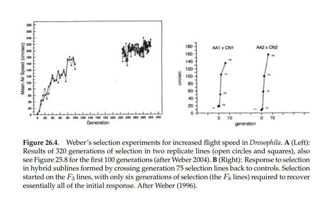
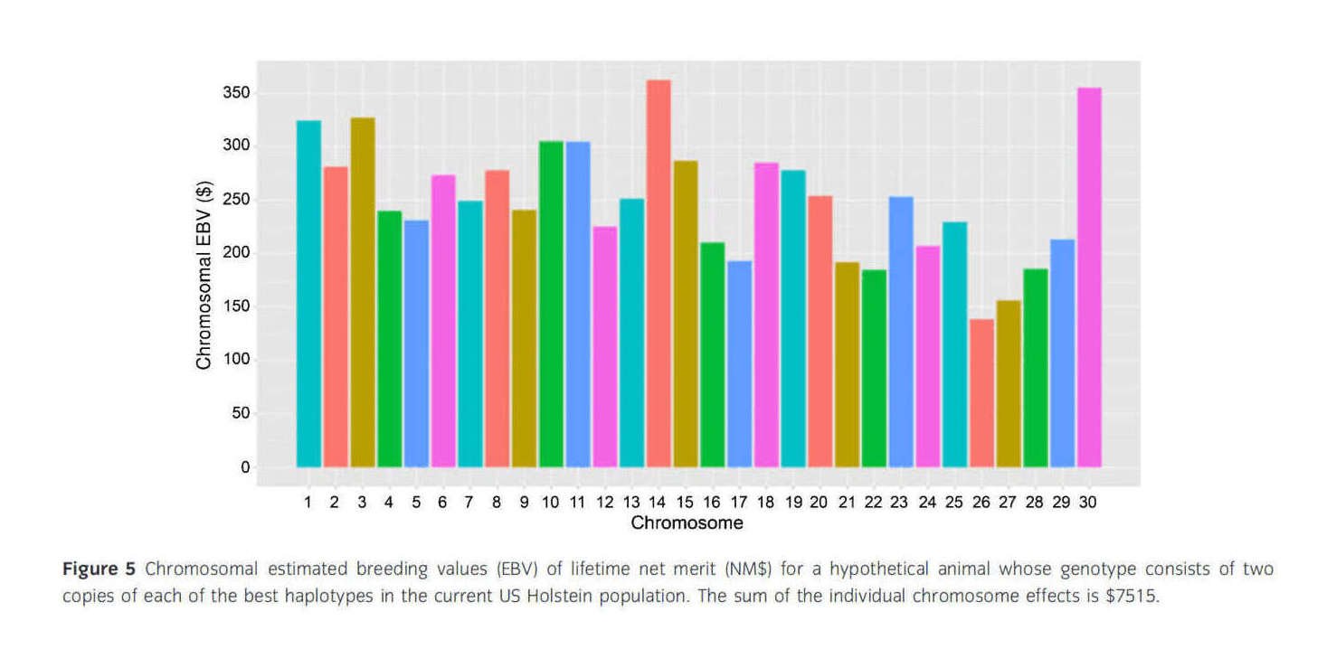
We have already seen that the initial response in the first generation depends on the PGS power and number of embryos, and the gain could be greatly increased by both PGSes approaching the upper bound of 80% variance and by “massive embryo selection” over hundreds of embryos generated from a starting donated egg & sperm; both would likely be available (and the latter is required) by the time of any IES program, but the Robertson limit implies that for a reasonable gain like 10 IQ points, the total gain could easily be in the hundreds or thousands (eg. 50 × 2 × 10 = <1,000 or <66SD). The limit is approached with optimal selection intensities (there is a specific fraction which maximizes the gain by losing the fewest beneficial alleles due to the shrinking Ne over time) & increasingly large Ne (Walsh & Lynch2018 describe a number of experiments which typically reach a fraction of the limit like 1⁄10–1⁄3, but give a striking example of a large-scale selective breeding experiment which approaches the limit: Weber’s increase of fruit fly flying speed by >85x in Weber1996/Weber2004/graph); with dominance or many rare or recessive variants, the gain could be larger than suggested by Robertson’s limit. Cole & VanRaden2011 offers an example of estimating limits to selection in Holstein cows, using the “net merit” index (“NM$”), an index of dozens of economically-weighted traits expressing the total lifetime profit compared to a baseline of a cow’s offspring. Among (selected for breeding) Holstein cows, the net merit 2004 SD was $336.6$1912004; the 2010–201115ya net merit average was ~$236.84$1502010; and the 201115ya maximum across the whole US Holstein population (best of ~10 million?) was $2,465.47$1,5882011 (+7SD). Cole & VanRaden2011 estimate that a lower bound on net merit, if one optimized just the best 30 haplotypes, would yield a final net merit gain of $11,667.51$7,5152011 (>36SD); if one optimized all haplotypes, then the expected gain is $30,433.33$19,6022011 (+97SD); and the upper bound on the expected gain is $135,770.03$87,4492011 (<436SD). Even in the lower bound scenario, optimizing 1 out of the 30 cow chromosomes can yield improvements of 1–2SD (Cole & VanRaden2011 Figure 5) (Crow2010 suggests that narrowsense heritability doesn’t become exhausted and dominated by epistasis in breeding scenarios because rare variants make little contribution to heritability estimates initially but as they become more common, they make a larger contribution to observed heritability, thereby offsetting the loss of genetic diversity from initially-common variants being driven to fixation by the selection—that is, the baseline heritability estimates ignore the potential by the ‘dark matter’ of millions of rare variants which affect the trait being selected for.)
Paradoxically, the more genes involved and thus the worse our polygenic scores are at a given fraction of heritability, the longer selection can operate and the more the potential gains.
It’s true that a polygenic score might be able to predict only a small fraction of variance, but this is not because it has identified no relevant variants but in large part because of the Central Limit Theorem: with thousands of genes with additive effects, they sum up to a tight bell curve, and it’s 5001 steps forward, 4999 steps backwards, and our prediction’s performance is being driven by our errors on a handful of variants on net—which gives little hint as to what would happen if we could take all 10000 steps forward. This is admittedly counterintuitive; an example of incredulity is sociologist Catherine Bliss’s attempt to scoff at behavioral genetics GWASes (quoting from a Nature review):
She notes, for example, a special issue of the journal Biodemography and Social Biology from 201412ya concerning risk scores. (These are estimates of how much a one-letter change in the DNA code, or SNP, contributes to a particular disease.) In the issue, risk scores of between 0% and 3% were taken as encouraging signs for future research. Bliss found that when risk scores failed to meet standards of statistical-significance, some researchers—rather than investigate environmental influences—doggedly bumped up the genetic significance using statistical tricks such as pooling techniques and meta-analyses. And yet the polygenic risk scores so generated still accounted for a mere 0.2% of all variation in a trait. “In other words,” Bliss writes, “a polygenic risk score of nearly 0% is justification for further analysis of the genetic determinism of the traits”. If all you have is a sequencer, everything looks like an SNP.
But this ignores the many converging heritability estimates which show SNPs collectively matter, the fact that one would expect polygenic scores to account for a low percentage of variance due to the CLT & power issues, that a weak polygenic score has already identified with high posterior probability many variants and the belief it hasn’t reflects arbitrary NHST dichotomization, that a low percentage polygenic score will increase considerably with sample sizes, and that this has already happened with other traits (height being a good case in point, going from ~0% in initial GWASes to ~40% by 2017, exactly as predicted based on power analysis of the additive architecture). It may be counterintuitive, but a polygenic score of “nearly 0%” is another way of saying it isn’t 0%, and is justification for further study and use of “statistical tricks”.
An analogy here might be siblings and height: siblings are ~50% genetically related, and no one doubts that height is largely genetic, yet you can’t predict one sibling’s height all that well from another’s, even though you can predict almost perfectly with identical twins—who are 100% genetically related; in a sense, you have a ‘polygenic score’ (one sibling’s height) which has exactly identified ‘half’ of the genetic variants affecting the other sibling’s height, yet there is still a good deal of error. Why? Because the sum total of the other half of the genetics is so unpredictable (despite still being genetic).
So the total potential gain has more to do with the heritability vs number of alleles, which makes sense—if a trait is mostly caused by a single gene which half the population already has, we would not expect to be able to make much difference; but if it’s mostly caused by a few dozen genes, then few people will have the maximal value; and if by a few hundred or a few thousand, then probably no one will have ever had the maximal value and the gain could be enormous.
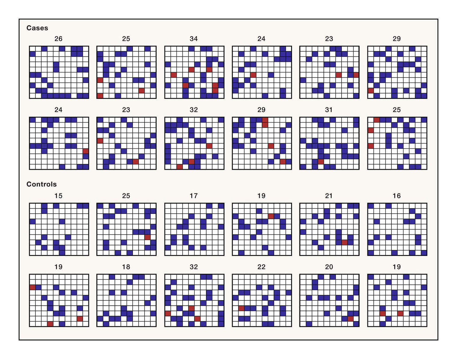
Individual differ greatly by genetic risk. But can you easily tell—without access to the total PGS sum!—which of these has the highest risk, and which the lowest risk? (Visualization from Wray et al 2018, “Figure 1. Between Individual Genetic Heterogeneity under a Polygenic Model”)
As Hsu2014 explains in a simple coin-flip model: if you flip a large number of coins and sum them, most of the heads and tails cancel out, and the sum is determined by the slight excess of heads or the slight excess of tails. If you were able to measure even a large fraction of, say, 50 coins to find out how they landed, you would still have great difficulty predicting whether the overall sum turns out to be +5 heads or -2 tails. However, that doesn’t mean that the coin flips don’t affect the final sum (they do), or that the result can’t eventually be ‘predicted’ if you could measure more coins more accurately; and consider: what if you could reach out and flip over each coin? Instead of a large collection of outcomes like +4 or -3, or +8, or -1, all distributed around 0, you could have an outcome like +50—and you would have to flip a set of 50 coins for a long time indeed to ever see a +50 by chance. In this analogy, alleles are coins, their frequency in the population is the odds of coming up heads, and reaching in to flip over some coins to heads is equivalent to using selection to make alleles more frequent and thus more likely to be inherited.
In high-dimensional spaces, there is almost always a point near a goal, and extremely high/low value points can be found despite many overlapping constraints or dimensions; Yong et al 2020 demonstrates that with UKBB PGSes, the overlap in SNP regions is low enough that it is possible to have a genome which is extremely low on many health risks simultaneously, by optimizing them all to extremes. For a concrete example of this, consider the case of basketball player Shawn Bradley who, at a height of 7 feet 6 inches, is at the 99.99999th percentile (less than 1 in a million / +8.6SD). Bradley has none of the usual medical or monogenic disorders which cause extreme height, and indeed turns out to have an unusual height PGS—using the GIANT PGS with only 2900 SNPs (predicting ~21–24% of variance), his PGS2.9k is +4.2SD (Sexton et al 2018), indicating much of his height is being driven by having a lot of height-boosting common variants. What is ‘a lot’ here? Sexton et al 2018 dissects the PGS2.9k and finds that even in an outlier like Bradley, the heterozygous increasing/decreasing variants are almost exactly offset (621 vs 634 variants, yielding net effects of +15.12 vs -15.27), but the homozygous variants don’t quite offset (465 variants vs 267 variants, nets of +25.89 vs -15.42), and all 4 categories combined leaves a residue of +10.32; that is, the part of his height affected by the 2900 SNPs is due almost entirely to just 198 homozygous variants, as the other ~2700 cancel out.
To put it a little more rigorously like Student1933 did in discussing the implication of the long-term Illinois maize/corn oil experiments, consider a simple binomial model of 10000 alleles with 1/0 unit weights at 50% frequency, explaining 80% of variance; the mean sum will be 10000*0.5=5000 with an SD of sqrt(10000*0.5*0.5)=50; if we observe a population IQ SD of 15, and each +SD is due 80% to having +50 beneficial variants, then each allele is worth ~0.26 points, and then, regardless of any ‘polygenic score’ we might’ve constructed explaining a few percentage of the 10000 alleles’ influence, the maximal gain over the average person is 0.26*(10000-5000)=1300 points/86SDs. If we then select on such a polygenic trait and we shift the population mean up by, say, 1 SD, then the average frequency of 50% need only increase to an average of 50.60% (as makes sense if the total gain from boosting all alleles to 100%, an increase of 50% frequency, is 86SD, so each SD requires less than 1% shift). A more realistic model with exponentially distributed weights gives a similar estimate.
This sort of upper bound is far from what is typically realized in practice, and the fact that frequencies of variants are far from fixation (reaching either 0% or 100%) can be seen in examples like the maize oil experiments where, after generations of intense selection, yielding enormous changes, up to apparent physical limits like ~0% oil composition, they tried reversing selection, and selection proceeded in the opposite direction without a problem—showing that countless genetic variants remained to select on.
We could also ask what the upper limit is by looking at an existing polygenic score and seeing what it would predict for a hypothetical individual who had the better version of each one. The Rietveld et al 2013 polygenic score for education-years is available and can be adjusted into intelligence, but for clarity I’ll use the Benyamin et al 2014 polygenic score on intelligence (codebook):
benyamin <- read.table("CHIC_Summary_Benyamin2014.txt", header=TRUE)
nrow(benyamin); summary(benyamin)
# [1] 1380158
#          SNP               CHR               BP            A1         A2
#  rs1000000 :      1   chr2   :124324   Min.   :     9795   A:679239   C:604939
#  rs10000010:      1   chr1   :107143   1st Qu.: 34275773   C: 96045   G:699786
#  rs10000012:      1   chr6   :100400   Median : 70967101   T:604874   T: 75433
#  rs10000013:      1   chr3   : 98656   Mean   : 79544497
#  rs1000002 :      1   chr5   : 93732   3rd Qu.:114430446
#  rs10000023:      1   chr4   : 89260   Max.   :245380462
#  (Other)   :1380152   (Other):766643
#     FREQ_A1            EFFECT_A1                  SE                   P
#  Min.   :0.0000000   Min.   :-1.99100e-01   Min.   :0.01260000   Min.   :0.00000361
#  1st Qu.:0.2330000   1st Qu.:-1.12000e-02   1st Qu.:0.01340000   1st Qu.:0.23060000
#  Median :0.4750000   Median : 0.00000e+00   Median :0.01480000   Median :0.48370000
#  Mean   :0.4860482   Mean   : 2.30227e-06   Mean   :0.01699674   Mean   :0.48731746
#  3rd Qu.:0.7330000   3rd Qu.: 1.12000e-02   3rd Qu.:0.01830000   3rd Qu.:0.74040000
#  Max.   :1.0000000   Max.   : 2.00000e-01   Max.   :0.06760000   Max.   :1.00000000
Many of these estimates come with large p-values reflecting the relatively large standard error compared to the unbiased MLE estimate of its average additive effect on IQ points, and are definitely not genome-wide statistically-significant. Does this mean we cannot use them? Of course not! From a Bayesian perspective, many of these SNPs have high posterior probabilities; from a predictive perspective, even the tiny effects are gold because there are so many of them; from a decision perspective, the expected value is still non-zero as on average each will have its predicted effect—selecting on all the 0.05 variants will increase by that many 0.05s etc. (It’s at the extremes that the MLE estimate is biased.)
We can see that over a million have non-zero point-estimates and that the overall distribution of effects looks roughly exponentially distributed. The Benyamin SNP data includes all the SNPs which passed quality-checking, but is not identical to the polygenic score used in the paper as that removed SNPs which were in linkage disequilibrium; leaving such SNPs in leads to double-counting of effects (two SNPs in LD may reflect just 1 SNP’s causal effect). I took the top 1000 SNPs and used SNAP to get a list of SNPs with an r2>0.2 & within 250-KB, which yielded ~1800 correlated SNPs, suggesting that a full pruning would leave around a third of the SNPs, which we can mimic by selecting a third at random.
The sum of effects (corresponding to our imagined population which has been selected on for so many generations that the polygenic score no longer varies because everyone has all the maximal variants) is the thoroughly absurd estimate of +6k SD over all SNPs and +5.6k SD filtering down to p < 0.5 and +3k adjusting for existing frequencies (going from minimum to maximum); halving for symmetry, that is still thousands of possible SDs:
## simulate removing the 2/3 in LD
benyamin <- benyamin[sample(nrow(benyamin), nrow(benyamin)*0.357),]
sum(abs(benyamin$EFFECT_A1)>0)
# [1] 491497
sum(abs(benyamin$EFFECT_A1))
# [1] 6940.7508
with(benyamin[benyamin$P<0.5,], sum(abs(EFFECT_A1)))
# [1] 5614.1603
with(benyamin[benyamin$P<0.5,], sum(abs(EFFECT_A1)*FREQ_A1))
# [1] 2707.063157
with(benyamin[benyamin$EFFECT_A1>0,], sum(EFFECT_A1*FREQ_A1)) + with(benyamin[benyamin$EFFECT_A1<0,], abs(sum(EFFECT_A1*(1-FREQ_A1))))
# [1] 3475.532912
hist(abs(benyamin$EFFECT_A1), xlab="SNP intelligence estimates (SDs)", main="Benyamin et al 2014 polygenic score")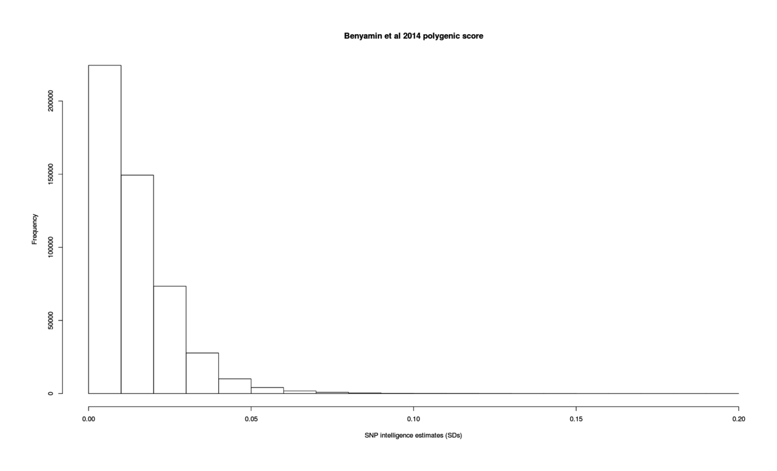
The betas/effect-sizes of the Benyamin et al 2014 polygenic score for intelligence, illustrating the many thousands of variants available for selection on.
One might wonder about what if we were to start with the genome of someone extremely intelligent, such as a John von Neumann, perhaps cloning cells obtained from grave-robbing the Princeton Cemetary? (Or so the joke goes–in practice, a much better approach would be to instead investigate buying up von Neumann memorabilia which might contain his hair or saliva, such as envelopes & stamps.) Cloning is a common technique in agriculture and animal breeding, with the striking recent example of dozens of clones of a champion polo horse, as a way of getting high performance quickly, reintroducing top performers into the population for additional selection, and allowing large-scale reproduction through surrogacy. (For a useful scenario for applying cloning techniques, see “Dog Cloning For Special Forces: Breed All You Can Breed”.)
Would selection or editing then be ineffective because one is starting with such an excellent baseline? Such clones would be equivalent to an “identical twin raised apart”, sharing 100% of genetics but none of the shared-environment or non shared-environment, and thus the usual ~80% of variance in the clones’ intelligence would be predictable from the original’s intelligence; however, since the donor is chosen for his intelligence, regression to the mean will kick in and the clones will not be as intelligent as the original.
How much less? If we suppose von Neumann was 170 (+4.6SDs), then his identical-twin/embryos would regress to the genetic mean of 4.6 × 0.8 = 3.68 SDs or IQ 155, with a modest chance to match or exceed him if they got lucky with the remaining 20% variance. (His siblings would’ve been lower still than this, of course, as they would only be 50% related even if they did have the same shared-environment.) With <0.2 IQ points per beneficial allele and a genetic contribution of +55, then von Neumann would’ve only needed (155 − 100) / (<0.2) = >275 positive variants compared to the average person; but he would still have had thousands of negative variants left for selection to act against.
Having gone through the polygenic scores and binomial/gamma models, this conclusion will not come as a surprise: since existing differences in intelligence are driven so much by the effects of thousands of variants, the CLT/standard deviation of a binomial/gamma distribution implies that those differences represent a net difference of only a few extra variants, as almost everyone has, say, 4,990 or 5,001 or 4,970 or 5,020 good variants and no one has extremes like 9,000 or 3,000 variants—even a von Neumann only had slightly better genes than everyone else, probably no more than a few hundred. Hence, anyone who does get thousands of extra good variants will be many SDs beyond what we currently see.
Alternately to trying to directly calculate a ceiling from polygenic scores, from a population genetics perspective, Robertson1960 shows that for additive selection, the total possible gain from artificial selection is equivalent to twice the ‘effective’/breeding population times the gain in the first generation, reflecting the tradeoff in a smaller effective population—randomly losing useful variants by stringent selection. (Hill1982 considers the case where new mutations arise, as of course they very gradually do, and finds a similar limit but multiplied by the rate of new useful mutations.) This estimate is more of a loose lower bound than an upper bound since it describes a pure selection program based on just phenotypic observations where it is assumed each generation ‘uses up’ some of the additive variance, whereas empirically selection programs do not always observe decreasing additive variance, we can directly examine or edit or synthesize genomes, so we don’t have to worry too much about losing variants permanently. If one considered an embryo selection program in a human population of millions of people and the polygenic scores yielding at least an IQ point or two, this also yields an estimate of an absurdly large total possible gain—here too the real question is not whether there is enough additive variance to select on, but what the underlying biology supports before additivity breaks down.
The major challenges to IES are how far the polygenic scores will be valid before breaking down.
Polygenic scores from GWASes draw most of their predictive power not from identifying the exact causal variants, but identifying SNPs which are correlated with causal variants and can be used to predict their absence or presence. With a standard GWAS and without special measures like fine-mapping, only perhaps 10% of SNPs identified by GWASes will themselves be causal. For the other 90%, since genes are inherited in ‘blocks’, a SNP might almost always be inherited along with an unknown causal variant; the SNPs are in “linkage disequilibrium” (LD) with the causal variants and are said to “tag” them. However, across many generations, the blocks are gradually broken up by chromosomal recombination and a SNP will gradually lose its correlation with its causal variant; this causes the original polygenic score to lose overall predictive power as more selection power is spent on increasing the frequency of SNPs which no longer tag their causal variant and are simply noise. This is unimportant for single selection steps because a single generation will change LD patterns only slightly, and in normal breeding programs, fresh data will continue to be collected and used to update the GWAS results and maintain the polygenic score’s efficacy while an unchanged polygenic score loses efficacy (eg. Neyhart et al 2016 show this in barley simulations); but in an IES program, one doesn’t want to stop every, say, 5 generations and wait a decade for the embryos to grow up and fresh data, so the polygenic score predictive power will degrade down to that lower bound and the genetic value will hit the corresponding ceiling. (So at a rough guess, a human intelligence GWAS polygenic score would degrade down to ~10% efficacy within 5-10 generations of selection, and the total gains would be upper bounded at 10% of the theoretical limit of so perhaps hundreds of SDs at most.)
Secondly, if all the causal variants were maxed out and driven to fixation, it’s unclear how much gain there would be because variants with additive effects within the normal human range may become non-additive beyond that. Thousands of SDs is meaningless, since intelligence reflects neurobiological traits like nerve conduction velocity, brain size, white matter integrity, metabolic demands etc., all of which must have inherent biological limits (although considerations from the scaling of the primate brain architecture suggest that the human brain could be increased substantially, similar to the increase from Australopithecus to humans, before gains disappear; see Hofman2015); so while it’s reasonable to talk about boosting to 5-10SDs based on additive variants, beyond that there’s no reason to expect additivity to hold. Since the polygenic score only becomes uninformative hundreds of SDs beyond where other issues will take over, we can safely say that the polygenic scores will not ‘run dry’ during an IES project, much less normal embryo selection—additivity will run out before the polygenic score’s information does.
But there is one reason to suspect that an appropriate increase in size, together with other comparatively minor changes in structure, might lead to a large increase in intelligence. The evolution of modern man from non-tool-making ancestors has presumably been associated with and dependent on a large increase in intelligence, but has been completed in what is on an evolutionary scale a rather short time—at most a few million years. This suggests that the transformation which provided the required increase in intelligence may have been growth in size with relatively little increase in structural complexity—there was insufficient time for natural selection to do more…To ask oneself the consequence of building such an intelligence is a little like asking an Australopithecine what kind of questions Newton would ask himself and what answers he would give…I suspect that if our species survives, someone will try it and see.
—pg76, “Eugenics and Utopia”, On Evolution, John Maynard Smith 1972