Daily ratings:
mp <- na.omit(read.csv("~/selfexperiment/mp.csv", colClasses=c("Date", "integer")))(I am not using any productivity factors which might improve substantially on my MP self-ratings because in the analyses I try periodically with a large set of variables eg. Git commits & number of emails sent, as of May 2018, I still haven’t found any clear ‘productivity’ factor, to my disappointment.)
Query Mnemosyne spaced repetition logs (see Treadmill), get grades recorded each day (which reflects memory retrieval that day) and the next future grade for each card (reflects memory encoding/increase in memorization that day), along with ‘easiness’ and hour/day covariates; then fit a Bayesian multilevel model with random effects for each card and day regressing on current & future grade; finally, extract the two random-effects for each day and sum them to get an index variable of my memory performance that day:
target <- "~/doc/mnemosyne/default.db"
library(sqldf)
# .schema log
# CREATE TABLE log(
#         _id integer primary key autoincrement,
#         event_type integer,
#         timestamp integer,
#         object_id text,
#         grade integer,
#         easiness real,
#         acq_reps integer,
#         ret_reps integer,
#         lapses integer,
#         acq_reps_since_lapse integer,
#         ret_reps_since_lapse integer,
#         scheduled_interval integer,
#         actual_interval integer,
#         thinking_time integer,
#         next_rep integer,
#         scheduler_data integer
#     );
grades <- sqldf("SELECT timestamp,object_id,grade,easiness,thinking_time,actual_interval,(SELECT grade \
                 FROM log AS log2 WHERE log2.object_id = log.object_id AND log2.timestamp > log.timestamp \
                 ORDER BY log2.timestamp DESC LIMIT 1) AS grade_future FROM log WHERE event_type==9;",
                dbname=target,
                method = c("integer", "factor","integer","numeric","integer","integer", "integer"))
grades$timestamp <- as.POSIXct(grades$timestamp, origin = "1970-01-01", tz = "EST")
grades$thinking_time.log <- log1p(grades$thinking_time); grades$thinking_time <- NULL
colnames(grades) <- c("Timestamp", "ID", "Grade", "Easiness", "Interval.length", "Grade.future",
                       "Thinking.time.log")
## extract the temporal covariates from the timestamp
grades$WeekDay <- as.factor(weekdays(grades$Timestamp))
grades$Hour    <- as.factor(as.numeric(format(grades$Timestamp, "%H")))
grades$Date    <- as.Date(grades$Timestamp)

## multilevel model: mean-field variational inference rather than MCMC to avoid days of computation
library(brms)
mb <- brm(cbind(Grade,Grade.future) ~ (1|ID) + (1|Date.int) + WeekDay + Hour + Easiness, data=grades, algorithm="mean")
summary(mb)
r <- as.data.frame(ranef(mb)$Date.int)
averageGrade <- r$Estimate.Grade_Intercept + r$Estimate.Gradefuture_Intercept
dates <- as.Date(as.integer(rownames(r)), origin = "1970-01-01")
gradeDaily <- data.frame(Date=dates, Mnemosyne.performance=averageGrade)
Zeo code largely borrowed from most-recent style of analysis in CO2/ZMA; for more details, see those, but the idea is to transform the variables into more Gaussian-looking variables for stabler model-fitting, specify a plausible amount of measurement error, define 2 latent variables for good and bad sleep (oddly, they don’t seem to be negations of each other), and like the Mnemosyne code, extract the latent variables for each day and sum into a single sleep quality score:
zeo <- read.csv("https://gwern.net/doc/zeo/gwern-zeodata.csv")
zeo$Date <- as.Date(sapply(strsplit(as.character(zeo$Rise.Time), " "), function(x) { x[1] }), format="%m/%d/%Y")
zeo <- subset(zeo, select=c("Date", "ZQ", "Total.Z", "Time.to.Z", "Time.in.Wake", "Time.in.REM",
    "Time.in.Light", "Time.in.Deep", "Awakenings", "Morning.Feel"))

zeo$Total.Z.2 <- zeo$Total.Z^2
zeo$ZQ.2 <- zeo$ZQ^2
zeo$Time.in.REM.2 <- zeo$Time.in.REM^2
zeo$Time.in.Light.2 <- zeo$Time.in.Light^2
zeo$Time.in.Wake.log <- log1p(zeo$Time.in.Wake)
zeo$Time.to.Z.log <- log1p(zeo$Time.to.Z)

model1 <- '
 ## single-indicator measurement error model for each sleep variable assuming decent reliability:
 ZQ.2_latent =~ 1*ZQ.2
 ZQ.2 ~~ 0.7*ZQ.2
 Total.Z.2_latent =~ 1*Total.Z.2
 Total.Z.2 ~~ 0.7*Total.Z.2
 Time.in.REM.2_latent =~ 1*Time.in.REM.2
 Time.in.REM.2 ~~ 0.7*Time.in.REM.2
 Time.in.Light.2_latent =~ 1*Time.in.Light.2
 Time.in.Light.2 ~~ 0.7*Time.in.Light.2
 Time.in.Deep_latent =~ 1*Time.in.Deep
 Time.in.Deep ~~ 0.7*Time.in.Deep
 Time.to.Z.log_latent =~ 1*Time.to.Z.log
 Time.to.Z.log ~~ 0.7*Time.to.Z.log
 Time.in.Wake.log_latent =~ 1*Time.in.Wake.log
 Time.in.Wake.log ~~ 0.7*Time.in.Wake.log
 Awakenings_latent =~ 1*Awakenings
 Awakenings ~~ 0.7*Awakenings

 GOOD_SLEEP =~ ZQ.2_latent + Total.Z.2_latent + Time.in.REM.2_latent + Time.in.Light.2_latent + Time.in.Deep_latent + Morning.Feel
 BAD_SLEEP  =~ Time.to.Z.log_latent + Time.in.Wake.log_latent + Awakenings_latent
 '
## Fit Bayesian SEM:
library(blavaan)
s1 <- bsem(model1, n.chains=8, test="none", burnin=10000, sample=10000,
    dp = dpriors(nu = "dnorm(0,1)", alpha = "dnorm(0,1)", beta = "dnorm(0,200)"),
    jagcontrol=list(method="rjparallel"), fixed.x=FALSE, data=scale(zeo[-1])); summary(s1)
sleepIndex <- predict(s1)[,9] - predict(s1)[,10] # GOOD_SLEEP - BAD_SLEEP
zeo$Sleep.performance <- sleepIndex
Merge the 3 datasets, restrict down to the ABABA time-range, classify by Bacopa status:
df <- merge(zeo, merge(gradeDaily, mp, all=TRUE), all=TRUE)
df <- df[!is.na(df$Date),]
df <- df[df$Date>=as.Date("2014-06-28") & df$Date<=as.Date("2015-09-04"),]
df$Date.int <- as.integer(df$Date)

df$Bacopa <- FALSE
df[df$Date>=as.Date("2014-06-28") & df$Date<=as.Date("2014-09-25"),]$Bacopa <- FALSE
df[df$Date>=as.Date("2014-09-26") & df$Date<=as.Date("2014-12-19"),]$Bacopa <- TRUE
df[df$Date>=as.Date("2014-12-20") & df$Date<=as.Date("2015-03-19"),]$Bacopa <- FALSE
df[df$Date>=as.Date("2015-03-20") & df$Date<=as.Date("2015-06-05"),]$Bacopa <- TRUE
df[df$Date>=as.Date("2015-06-06") & df$Date<=as.Date("2015-09-04"),]$Bacopa <- FALSE

write.csv(df, row.names=FALSE, file="2018-05-17-gwern-bacopa.csv")
df <- read.csv("https://gwern.net/doc/nootropic/bacopa/2018-05-17-gwern-bacopa.csv")
# Date ZQ Total.Z Time.to.Z Time.in.Wake Time.in.REM
# Min. :2014-06-28 Min. : 14.00000 Min. : 70.0000 Min. : 1.00000 Min. : 0.00000 Min. : 12.0000
# 1st Qu.:2014-10-14 1st Qu.: 85.00000 1st Qu.:496.2500 1st Qu.: 7.00000 1st Qu.: 12.00000 1st Qu.:138.0000
# Median :2015-01-30 Median : 95.00000 Median :544.0000 Median :20.00000 Median : 23.00000 Median :163.0000
# Mean :2015-01-30 Mean : 93.11521 Mean :530.2465 Mean :19.64286 Mean : 29.20507 Mean :157.4816
# 3rd Qu.:2015-05-18 3rd Qu.:103.00000 3rd Qu.:579.0000 3rd Qu.:27.00000 3rd Qu.: 37.00000 3rd Qu.:183.0000
# Max. :2015-09-04 Max. :129.00000 Max. :682.0000 Max. :95.00000 Max. :167.00000 Max. :263.0000
# NA's :1 NA's :1 NA's :1 NA's :1 NA's :1
# Time.in.Light Time.in.Deep Awakenings Morning.Feel Total.Z.2 ZQ.2 Time.in.REM.2
# Min. : 38.0000 Min. : 5.0000 Min. : 0.000000 Min. :0.000000 Min. : 4900.0 Min. : 196.000 Min. : 144.00
# 1st Qu.:292.0000 1st Qu.: 48.0000 1st Qu.: 4.000000 1st Qu.:2.000000 1st Qu.:246264.2 1st Qu.: 7225.000 1st Qu.:19044.00
# Median :317.0000 Median : 57.0000 Median : 6.000000 Median :3.000000 Median :295936.0 Median : 9025.000 Median :26569.00
# Mean :313.9516 Mean : 59.3318 Mean : 6.341014 Mean :2.562212 Mean :287184.9 Mean : 8915.078 Mean :26341.23
# 3rd Qu.:344.7500 3rd Qu.: 69.0000 3rd Qu.: 8.000000 3rd Qu.:3.000000 3rd Qu.:335241.0 3rd Qu.:10609.000 3rd Qu.:33489.00
# Max. :459.0000 Max. :142.0000 Max. :16.000000 Max. :4.000000 Max. :465124.0 Max. :16641.000 Max. :69169.00
# NA's :1 NA's :1 NA's :1 NA's :1 NA's :1 NA's :1 NA's :1
# Time.in.Light.2 Time.in.Wake.log Time.to.Z.log Sleep.performance Mnemosyne.performance MP
# Min. : 1444.0 Min. :0.000000 Min. :0.6931472 Min. :-1.8207928 Min. :-0.81207471 Min. :1.000000
# 1st Qu.: 85264.0 1st Qu.:2.564949 1st Qu.:2.0794415 1st Qu.:-0.1382757 1st Qu.:-0.08138984 1st Qu.:3.000000
# Median :100489.0 Median :3.178054 Median :3.0445224 Median : 0.2507222 Median : 0.02087041 Median :3.000000
# Mean :100831.6 Mean :3.091542 Mean :2.6811233 Mean : 0.2215090 Mean : 0.00790124 Mean :3.262069
# 3rd Qu.:118852.8 3rd Qu.:3.637586 3rd Qu.:3.3322045 3rd Qu.: 0.6038839 3rd Qu.: 0.12563885 3rd Qu.:4.000000
# Max. :210681.0 Max. :5.123964 Max. :4.5643482 Max. : 1.8661274 Max. : 1.68682336 Max. :4.000000
# NA's :1 NA's :1 NA's :1 NA's :1 NA's :77
# Date.int Bacopa
# Min. :16249.0 Mode :logical
# 1st Qu.:16357.5 FALSE:271
# Median :16465.0 TRUE :164
# Mean :16465.4 NA's :0
# 3rd Qu.:16573.5
# Max. :16682.0
cor(subset(df, select=c("Sleep.performance", "Mnemosyne.performance", "MP", "Bacopa")), use="pairwise.complete.obs")
# Sleep.performance Mnemosyne.performance MP Bacopa
# Sleep.performance 1.000000000000
# Mnemosyne.performance -0.008373508585 1.000000000000
# MP 0.019296978791 0.029580496779 1.00000000000
# Bacopa -0.013829613334 -0.083324462060 -0.02286848706 1.00000000000
library(gridExtra)
p1 <- qplot(Date, Mnemosyne.performance, color=Bacopa, data=df) + stat_smooth()
p2 <- qplot(Date, MP, color=Bacopa, data=df) + stat_smooth()
p3 <- qplot(Date, Sleep.performance, color=Bacopa, data=df) + stat_smooth()
grid.arrange(p1, p2, p3, ncol=1)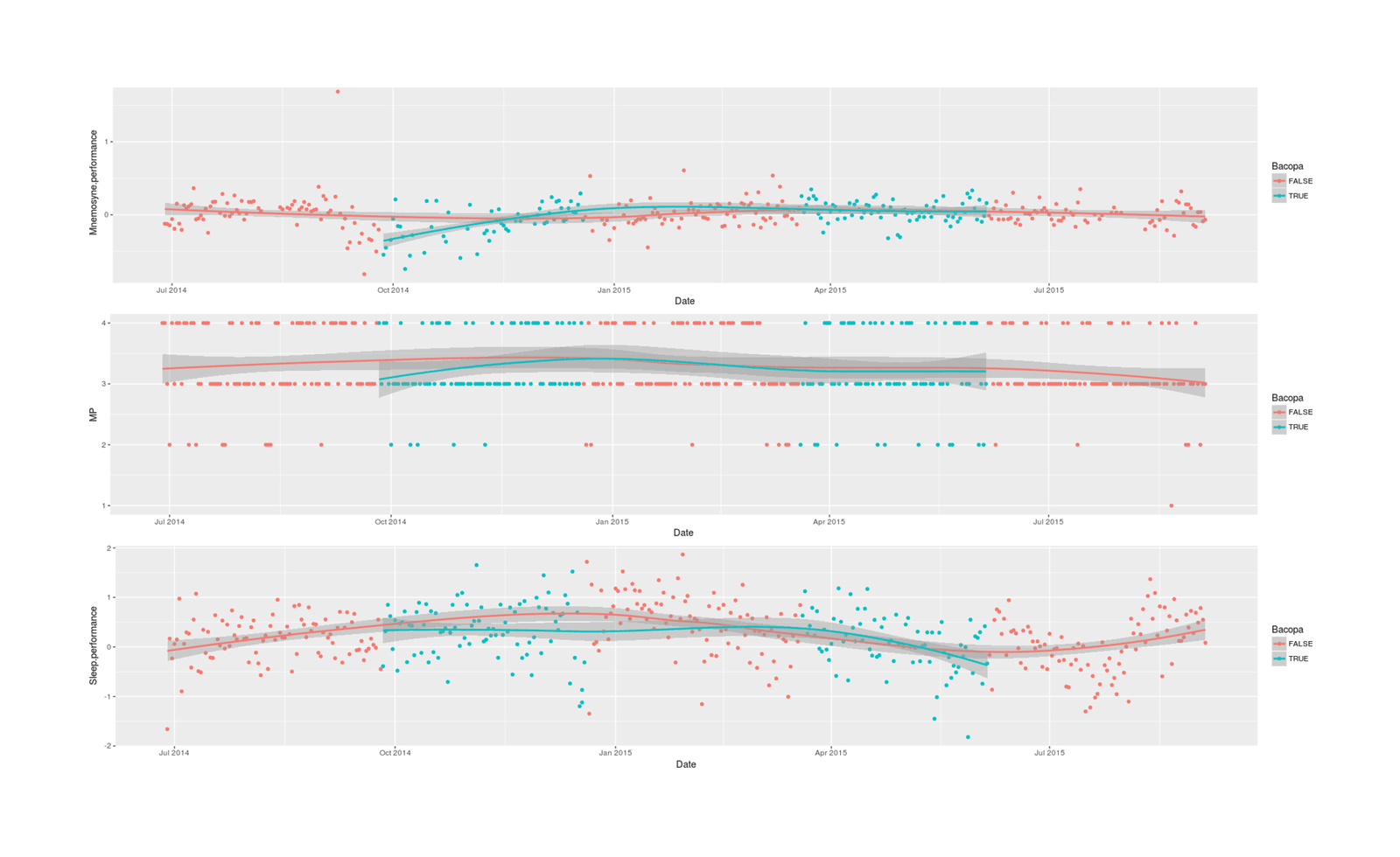
Graph of daily sleep, memory, and productivity self-ratings over time during Bacopa quasi-experiment
For analysis, the baseline linear model and then a Bayesian model with a B-spline to model the time-series/autocorrelation aspect:
summary(lm(cbind(Mnemosyne.performance, Sleep.performance, MP) ~ Bacopa, data=df))
# Response Mnemosyne.performance :
# ...Coefficients:
#                Estimate  Std. Error  t value Pr(>|t|)
# (Intercept)  0.02091904  0.01377171  1.51899  0.12966
# BacopaTRUE  -0.03534109  0.02256296 -1.56633  0.11816
#
# Residual standard error: 0.2061161 on 355 degrees of freedom
#   (78 observations deleted due to missingness)
# Multiple R-squared:  0.00686354,  Adjusted R-squared:  0.004065972
# F-statistic: 2.453396 on 1 and 355 DF,  p-value: 0.1181619
#
# Response Sleep.performance :
# ...Coefficients:
#                Estimate  Std. Error  t value   Pr(>|t|)
# (Intercept)  0.24477449  0.03711767  6.59455 1.5485e-10
# BacopaTRUE  -0.06054636  0.06081197 -0.99563    0.32011
#
# Residual standard error: 0.5555265 on 355 degrees of freedom
#   (78 observations deleted due to missingness)
# Multiple R-squared:  0.002784573, Adjusted R-squared:  -2.44843e-05
# F-statistic: 0.9912838 on 1 and 355 DF,  p-value: 0.320107
#
# Response MP :
# ...Coefficients:
#                Estimate  Std. Error  t value Pr(>|t|)
# (Intercept)  3.29464286  0.04072128 80.90716  < 2e-16
# BacopaTRUE  -0.03900376  0.06671595 -0.58462  0.55917
#
# Residual standard error: 0.6094603 on 355 degrees of freedom
#   (78 observations deleted due to missingness)
# Multiple R-squared:  0.0009618499,    Adjusted R-squared:  -0.001852342
# F-statistic: 0.3417855 on 1 and 355 DF,  p-value: 0.5591718
bacopa <- brm(cbind(Mnemosyne.performance, Sleep.performance, MP) ~ s(Date.int) + Bacopa, data=df); summary(bacopa)
#  Family: MV(gaussian, gaussian, gaussian)
#   Links: mu = identity; sigma = identity
#          mu = identity; sigma = identity
#          mu = identity; sigma = identity
# Formula: Mnemosyne.performance ~ s(Date.int) + Bacopa
#          Sleep.performance ~ s(Date.int) + Bacopa
#          MP ~ s(Date.int) + Bacopa
#    Data: df (Number of observations: 357)
# Samples: 4 chains, each with iter = 2000; warmup = 1000; thin = 1;
#          total post-warmup samples = 4000
#
# Smooth Terms:
#                                       Estimate Est.Error l-95% CI u-95% CI Eff.Sample Rhat
# sds(Mnemosyneperformance_sDate.int_1)     3.44      1.19     1.79     6.52        914 1.00
# sds(Sleepperformance_sDate.int_1)         3.30      1.43     1.24     6.89       1006 1.00
# sds(MP_sDate.int_1)                       0.80      0.85     0.02     3.13        871 1.01
#
# Population-Level Effects:
#                                  Estimate Est.Error l-95% CI u-95% CI Eff.Sample Rhat
# Mnemosyneperformance_Intercept      -0.02      0.02    -0.05     0.02       3372 1.00
# Sleepperformance_Intercept           0.28      0.05     0.19     0.39       2946 1.00
# MP_Intercept                         3.30      0.05     3.22     3.39       4000 1.00
# Mnemosyneperformance_BacopaTRUE      0.07      0.05    -0.02     0.16       3097 1.00
# Mnemosyneperformance_sDate.int_1     0.63      0.21     0.23     1.05       2168 1.00
# Sleepperformance_BacopaTRUE         -0.16      0.11    -0.40     0.04       2461 1.00
# Sleepperformance_sDate.int_1         1.23      0.47     0.39     2.21       1697 1.00
# MP_BacopaTRUE                       -0.07      0.08    -0.23     0.09       4000 1.00
# MP_sDate.int_1                      -0.15      0.23    -0.72     0.24       1444 1.00
#
# Family Specific Parameters:
#                                               Estimate Est.Error l-95% CI u-95% CI Eff.Sample Rhat
# sigma_Mnemosyneperformance                        0.19      0.01     0.17     0.20       4000 1.00
# sigma_Sleepperformance                            0.52      0.02     0.48     0.56       4000 1.00
# sigma_MP                                          0.61      0.02     0.57     0.66       4000 1.00
# rescor(Mnemosyneperformance,Sleepperformance)    -0.00      0.05    -0.11     0.10       4000 1.00
# rescor(Mnemosyneperformance,MP)                   0.02      0.05    -0.09     0.12       4000 1.00
# rescor(Sleepperformance,MP)                      -0.01      0.05    -0.11     0.09       4000 1.00
mean(posterior_samples(bacopa, "Mnemosyneperformance_BacopaTRUE")[,1] > 0)
# [1] 0.93025
mean(posterior_samples(bacopa, "Sleepperformance_BacopaTRUE")[,1] < 0)
# [1] 0.94525
mean(posterior_samples(bacopa, "MP_BacopaTRUE")[,1] < 0)
# [1] 0.803
Unsurprisingly given a de facto sample size n = 5 due to the long-term chronic effects forcing a small ABABA quasi-experimental design, the results are largely inconclusive; using multilevel Mnemosyne scores and latent sleep indexes can help reduce measurement error but can only do so much.
The strongest result, in terms of posterior probability of a nonzero correlation between Bacopa & the 3 variables, is, perhaps as one would predict based on the Bacopa literature, on my Mnemosyne memory performance: a 0.07 (95% credible interval: -0.02-0.16) SD increase in retention, P = 0.93. If real & causal, that would be a small effect, but perhaps worthwhile in some contexts like medical school cramming (especially since it comes on top of an already quite powerful memory enhancement intervention - spaced repetition). The other two estimated correlations, unfortunately, are negative and also of similar posterior probability (P = 0.95, P = 0.80).